The Nature of Code — Flow Fields

What is a “flow field”? You may have heard of the term or seen them before but never understood what it is. Let me explain.

The Vector Field

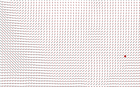
A flow field is based around a grid of vectors. These vectors, as you would expect, have a magnitude and direction. You can arrange them in a grid like so, with a position — the red dot — and the magnitude and direction — the black line

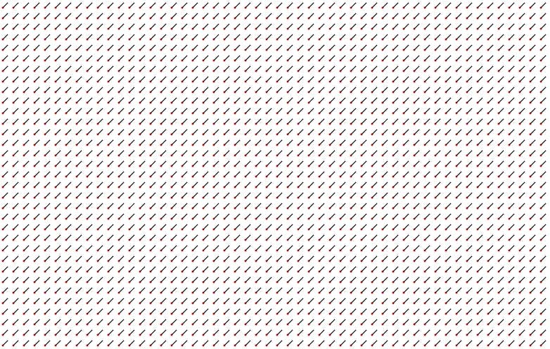
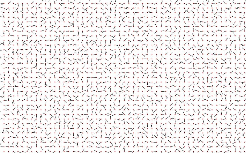
Currently, this grid contains only identical vectors. We need to add some randomness to the angle to make it more interesting and more importantly, different every time. If we choose a random angle for each vector, however, we end up with a completely scattered and unorganized mess.

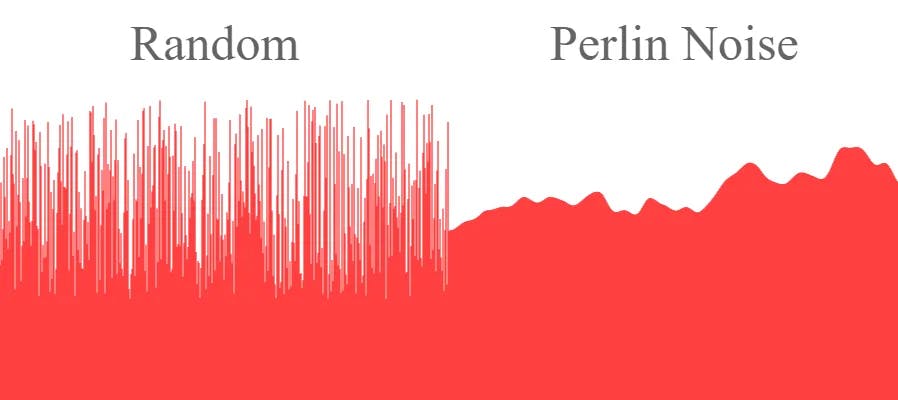
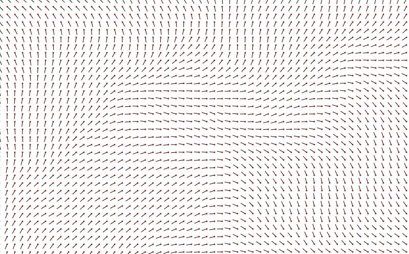
It seems we have to completely redefine what we call random. This is where we can introduce Perlin noise. It provides a more organic appearance as it produces a smoother progression of random numbers. Here is a comparison of the two side by side. It is easy to see how they differ from each other.

Implementing this into our code changes the vector field from a random mess into something that can very visually flow and all relate to each other. By just looking at it you might already see how it relates to nature. I like to relate it to the flow of a river as it usually adopts the same sort of random pattern.

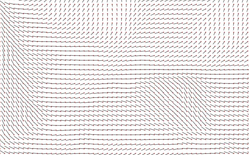
We can also apply the same principle to the magnitude of each vector to further diversify the vector field.

The Particle

Let’s create a particle to traverse this canvas. I decided to create it as an object to incorporate co-routines for thousands of particles. It needs to store a position and a velocity for now.

For it to follow the vector field, we need to get the vector at it’s current position and add it to the velocity of the particle. To do this we can get the current position on the screen — in pixels — and divide it by the gap between every vector. This gives you an index of which vector the particle is on. Given that the vectors are stored in a 2-D array, you can retrieve the vector and apply it to the velocity. We should also limit the velocity so the particles don’t speed up infinitely.

The wrap function makes sure that the particle never goes off the screen and just goes round the the other side, like a Taurus…or pac-man. This makes the final image look like one edge just flows onto the next.

class Particle {
    // initializes the starting variables    
    constructor() {      
        this.pos = createVector(random()  width, random()  height);
        this.vel = createVector(0, 0);    
    }        

    // finds nearest vector and add it to velocity    
    updateNearest() {          
        
        // finds vector index
        let i = floor(this.pos.x / gap);      
        let j = floor(this.pos.y / gap);            

        // adds vector to velocity      
        this.vel.x += dots[i][j].mag  cos(dots[i][j].theta);      
        this.vel.y += dots[i][j].mag  sin(dots[i][j].theta);            

        this.vel.setMag(3);            

        this.pos = p5.Vector.add(this.vel, this.pos);            

        this.wrap();    
    }           

    // makes sure the particle doesn't go off the screen    
    wrap() {          
        // checks edges      
        if (this.pos.x <= 0) {        
            this.pos.x = width-1;      
        }      
        if (this.pos.x >= width) {        
            this.pos.x = 1;      
        }      
        if (this.pos.y <= 0) {        
            this.pos.y = height-1;      
        }      
        if (this.pos.y >= height) {        
            this.pos.y = 1;      
        }    
    }        

    // displays the particle to the screen    
    draw() {      
        circle(this.pos.x, this.pos.y, 10);    
    }      
}

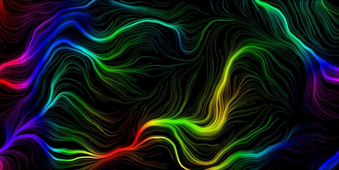
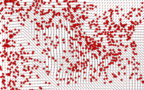
Adding many more particles, we see an interesting effect emerge. The particles seem to arrange themselves into a single line, taking all sorts of different paths from around it, some longer, some shorter.

The Visualization

The first thing we need to do is get rid of the vector field visualization and make the particles a bit smaller. Here’s where the art comes in. If we only refresh the screen once and make the dots slightly transparent. We get this result.

This is just the same boring color, however, if we want to spice things up we can change the color. For this, I want a color spectrum. Unluckily, RGB color isn’t very good at providing this. One such color mode that can do this is HSB. It has three values, just like RGB, except these values represent hue, saturation and brightness.

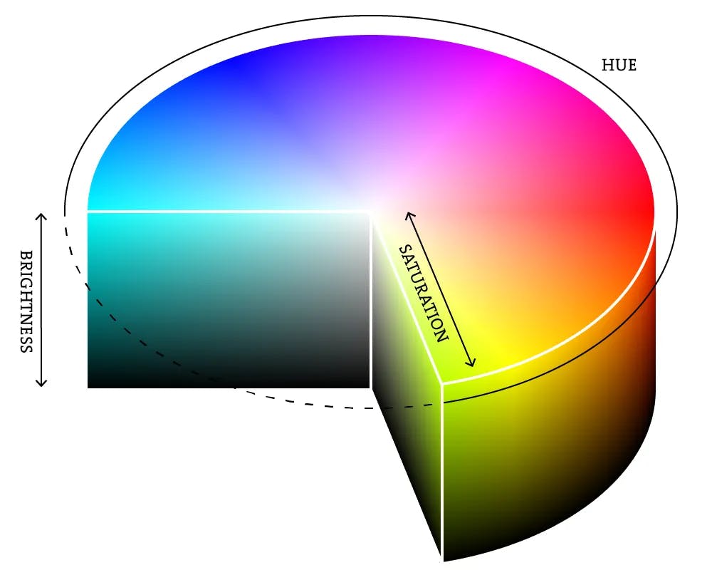
If we keep the brightness and saturation at full and only change the hue, we can cycle through the color spectrum easily. Then, we can apply Perlin noise based on the position of the particle to the hue, this will make the screen have regions of different colors that blend together. This is the final result.

Conclusion

There are endless possibilities of what can be made with flow fields, they are a process for generative art and any artist can bring their own take. What I have shown you today is just my take on flow fields and what I have managed to create. If you try to make this for yourself, experiment and make something new.